Simple Quadratic Regression Example

The purpose of this post is to give an example of how to visualize a quadratic linear regression and also how to find the values of the predictor variable which give you the min and max fitted values of your dependent variable. Given the curvilinear relationship between the independent and and dependent variable, it is not always obvious which values of the independent variable will produce the highest and lowest predicted values in the dependent variable. I will use the ‘mtcars’ data set that comes with your R installation.

head(mtcars)

##                    mpg cyl disp  hp drat    wt  qsec vs am gear carb
## Mazda RX4         21.0   6  160 110 3.90 2.620 16.46  0  1    4    4
## Mazda RX4 Wag     21.0   6  160 110 3.90 2.875 17.02  0  1    4    4
## Datsun 710        22.8   4  108  93 3.85 2.320 18.61  1  1    4    1
## Hornet 4 Drive    21.4   6  258 110 3.08 3.215 19.44  1  0    3    1
## Hornet Sportabout 18.7   8  360 175 3.15 3.440 17.02  0  0    3    2
## Valiant           18.1   6  225 105 2.76 3.460 20.22  1  0    3    1

library(ggplot2)
## plot base + points
plot.mgp.hp <- ggplot(mtcars, aes(x = hp, y = mpg)) + geom_point()
print(plot.mgp.hp)

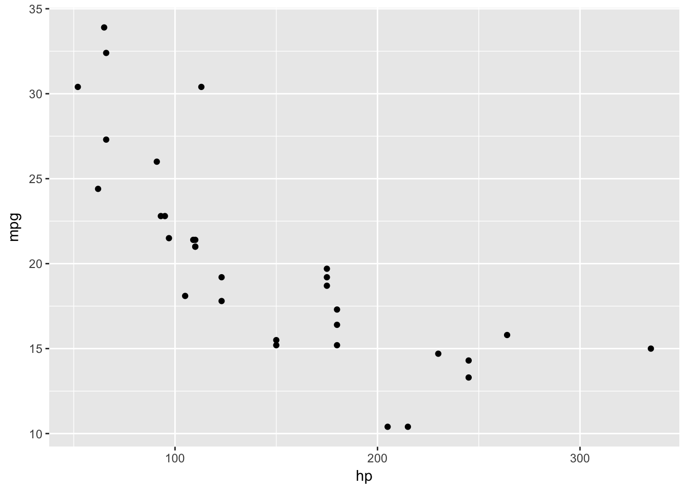
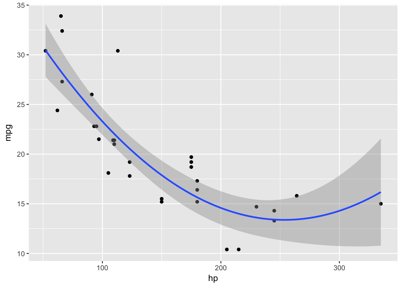
You can see in the intial graph above that there is a quadratic realtionship between the predictor hp and the outcome mpg. We can add the quadratic regression line into the plot itself. Using the poly method here is a time saver. It returns the main effect of the x variable along with the squared x variable.

formula <- y ~ poly(x, 2, raw = TRUE)
ggplot(mtcars, aes(x = hp, y = mpg)) +
      geom_point() +
      stat_smooth(method = "lm", formula = formula, size = 1)

Based on the curviture we can safely assume that the coefficient for hp is negative and coefficient for hp-squared is positive. Let’s check and see the actual regression table.

fit.mpg <- lm(mpg ~ poly(hp, 2), data = mtcars)
summary(fit.mpg)

## 
## Call:
## lm(formula = mpg ~ poly(hp, 2), data = mtcars)
## 
## Residuals:
##     Min      1Q  Median      3Q     Max 
## -4.5512 -1.6027 -0.6977  1.5509  8.7213 
## 
## Coefficients:
##              Estimate Std. Error t value Pr(>|t|)    
## (Intercept)    20.091      0.544  36.931  < 2e-16 ***
## poly(hp, 2)1  -26.046      3.077  -8.464 2.51e-09 ***
## poly(hp, 2)2   13.155      3.077   4.275 0.000189 ***
## ---
## Signif. codes:  0 '***' 0.001 '**' 0.01 '*' 0.05 '.' 0.1 ' ' 1
## 
## Residual standard error: 3.077 on 29 degrees of freedom
## Multiple R-squared:  0.7561, Adjusted R-squared:  0.7393 
## F-statistic: 44.95 on 2 and 29 DF,  p-value: 1.301e-09

As suspected, the main effect of hp is negative (-26.046) with a postive squared term (13.155). Both have a significant effect on mpg. Using this information we can use the model to predict the outcome and get the values of hp which produe the minimum and maximum values of the predicted mpg.

fitted.mpg <- fit.mpg$fitted.values

fitted.mpg.df <- as.data.frame(cbind(mtcars$hp, fitted.mpg))

min.index <- which.min(fitted.mpg.df$fitted.mpg)
max.index <- which.max(fitted.mpg.df$fitted.mpg)
min.mpg <- fitted.mpg.df[min.index,]
max.mpg <- fitted.mpg.df[max.index,]

print(min.mpg)

##             V1 fitted.mpg
## Camaro Z28 245   13.40805

print(max.mpg)

##             V1 fitted.mpg
## Honda Civic 52   30.45497

The maximum fitted mpg value was produced by the Honda civict with 52 horse power at 30.45 mpg while the Camaro Z28 with 245 horse power is a paltry 13.40 mpg.